Nonlinear Feedback Control in 3 Easy Steps
Many real autonomous systems are nonlinear, so we need more sophisticated nonlinear control methods to regulate them. In this article I start by showing how energy gives a much easier, and intuitive approach for reasoning about the stability of dynamic systems. Using this as a framework, I then introduce Lyapunov stability as a method for nonlinear analysis. Finally, I apply it to quaternions for orientation feedback control.
🧭 Navigation
Thinking Like a Physicist
The swinging pendulum on a grandfather clock moves back and forth in perpetuity (well, almost). Normally in control theory, when we talk about stability, we talk about system states where it is not moving. Or, in the case of trajectory tracking, the tracking error converges to zero. But a swinging pendulum isn’t exactly unstable. Its rhythmic motion is deliberately controlled at a rate of 1Hz. How can we reason about this kind of stability?
The pendulum of a grandfather clock swings back-and-forth, consistently, at 1Hz
Force?
If we took a Newtonian approach to the pendulum we would write the equations of motion as:
\[\begin{align} \overbrace{ml^2}^{I}\ddot{q} &= -mgl\cdot\sin(q) \tag{1a} \\ \ddot{q} &= -\tfrac{g}{l}\cdot\sin(q) \tag{1b} \end{align}\]where:
- $m\in\mathbb{R}^+$ is its mass (kg),
- $l\in\mathbb{R}^+$ is the length of the pendulum,
- $g\in\mathbb{R}$ is gravitational acceleration, and
- $q = [0, 2\pi]$ is the angle from vertical alignment
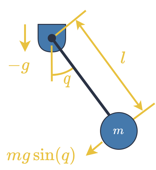
Physical modeling of a swinging pendulum.
Now, at this point, depending how much of a masochist you are, you can solve this nonlinear differential equation as:
\[q(t) = 2\cdot\arcsin\left(k\cdot sn(\omega t, k)\right) \tag{2}\]where:
- $k = \sin(\tfrac{1}{2}q(0))$,
- $\omega = \sqrt{\tfrac{g}{l}}$, and
- $sn(\cdot)$ is the Jacobi sine elliptic function.
Or we can do what most lazy academics do and abstract away all utility by assuming sin(q) ≈ q when q ≈ 0 such that:
\[\begin{align} \ddot{q} &\approx -\tfrac{g}{l}q \tag{3a}\\ \Longrightarrow q(t) &= A\cdot\cos(\omega t+\phi) \tag{3b} \end{align}\]where $A$ and $\phi$ are obtained from the initial conditions $q(0),~\dot{q}(0)$.
Either way, we end up with some complicated, trigonometric functions that:
- Don’t give us a clear method for reasoning about stability, and
- Don’t allow us to reason abstractly about other nonlinear systems.
No, Energy
Clearly, brute forcing mathematics won’t get us anywhere, which signifies we should change strategy. There is another physics paradigm we can appeal to instead: energy. The total energy in the system is:
\[E = \tfrac{1}{2}ml^2\dot{q}^2 + mgl\left(1 - \cos(q)\right) \tag{4}\]such that its time derivative is:
\[\begin{align} \dot{E} &= ml^2\dot{q}\ddot{q} + mgl\dot{q}\cdot \sin(q) \tag{5a} \\ &= -mgl\dot{q}\cdot\sin(q) + mgl\dot{q}\cdot\sin(q) \tag{5b}\\ &= 0. \tag{5c} \end{align}\]From the conservation of energy, its time derivative is zero. And, if we were to add a tiny bit of damping $b$:
\[ml^2\ddot{q} = -mgl\cdot\sin(q) - b\cdot\dot{q}^2 \tag{6}\]we would arrive at:
\[\dot{E} = -b\cdot\dot{q}^2 \le 0 ~\forall\dot{q}. \tag{7}\]which is non-increasing. We can conclude that a system is stable if:
- Its energy is non-increasing, and
- A better kind of stable if the energy is decreasing.
The Hamiltonian
The combination of $q$ and $\dot{q}$ is known as state space, and is very common in system dynamics. But Sir William Rowan Hamilton took an alternative approach using $q$ (the configuration), and momentum $p$. Combined, these form phase space. The momentum for the pendulum is:
\[p = ml^2\dot{q}. \tag{8}\]When combined with the configuration $q$ we have phase space. Furthermore, the Hamiltonian (i.e. total energy) of the system is:
\[\mathcal{H}(p,q) = \frac{1}{2}\frac{p}{(ml^2)} + mgl(1-\cos(q)). \tag{9}\]Since the Hamiltonian takes two inputs and maps them to a single (positive) output $\mathcal{H}:\mathbb{R}\times\mathbb{R}\mapsto\mathbb{R}^+$, we can visualise this as a 3D surface. Moreover, the time derivatives of the phase space coordinates are just partial derivatives of the Hamiltonian:
\[\dot{q} = \frac{\partial \mathcal{H}}{\partial p}~,~ \dot{p} = -\frac{\partial\mathcal{H}}{\partial q} \tag{10}\]These give a gradient vector which points in the direction that the system is changing, which we can plot on the energy surface. In the conservative case, we would see that a point on the phase space follows the same contour line (level set) along the surface, which corresponds to constant energy. A damped system will always move down from its current energy level.
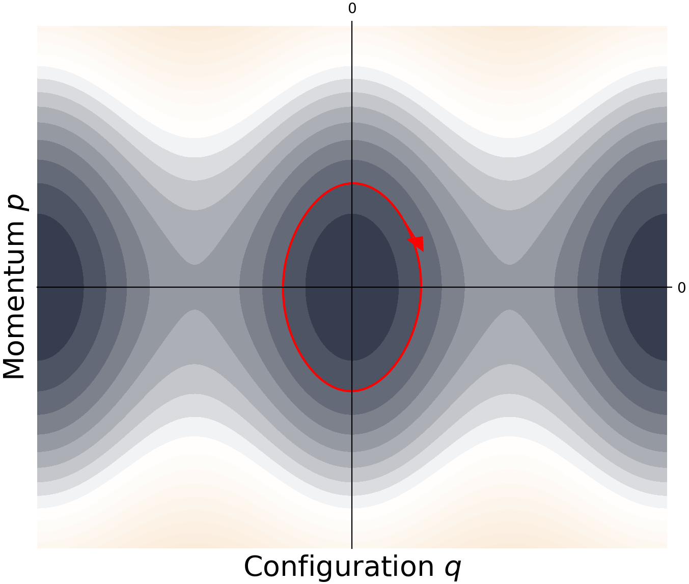
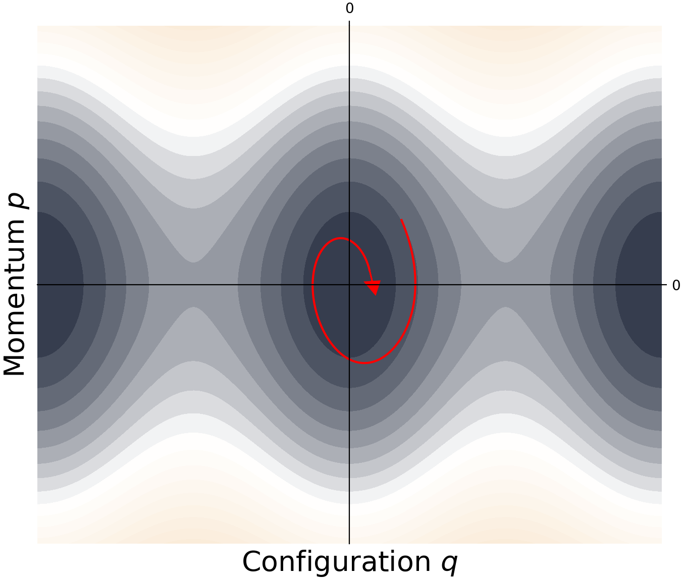
Phase portrait of a swinging pendulum. A conservative system remains on the same level set (contour line). A dissipative system always moves below its current level set.
Lyapunov Stability
Aleksandr Mikhailovich Lyapunov published a thesis on A General Problem of the Stability of Motion1. As you might have guessed, there are some mathematical definitions named after him that classify the different degrees of stability. But, from my experience, asking a mathematician about concepts in control theory is the very definition of masochism.
masochism: (noun)
Asking a mathematician about control theory.
I’ll circumvent the torture by giving a straightforward explanation. First, suppose we have a configuration $\mathbf{x}\in\mathbb{R}^n$, and some positive, scalar function that is zero for $\mathbf{x} = \mathbf{0}$:
\[V(\mathbf{x}) \ge 0 ~\forall\mathbf{x}\ne\mathbf{0} \quad,\quad V(\mathbf{0}) = 0. \tag{11}\]From this we may denote 3 levels of stability.
Stable in the Sense of Lyapunov:
If the Lyapunov function remains bounded with a finite region $\epsilon$, then the system is said to be stable:
For brevity, it is often referred to as Lyapunov stable. We can see from the pendulum example that the energy $E(q,\dot{q})$ is a natural choice for a Lyapunov function. In the undamped case, $\epsilon$ is its initial energy which remains constant (bounded) for all time.
Asymptotically Stable:
A system is asymptotically stable if we can show the time derivative of the Lyapunov function is non-increasing:
More precisely, it is monotonically non-increasing. It can decrease, or stay flat, but never increase. For the damped pendulum, its energy is decreasing with time, so it is asymptotically stable.
Exponentially Stable:
This is a more advanced case of the previous. If we can show that the time derivative is proportional to its current value, then it must be exponentially decreasing:
It is strictly decreasing, hence will converge to zero faster than the asymptotic case.
We can see that these 3 definitions form a nested hierarchy (see figure below):
- All exponentially stable systems are asymptotically stable, and
- All asymptotically stable systems are Lyapunov stable.
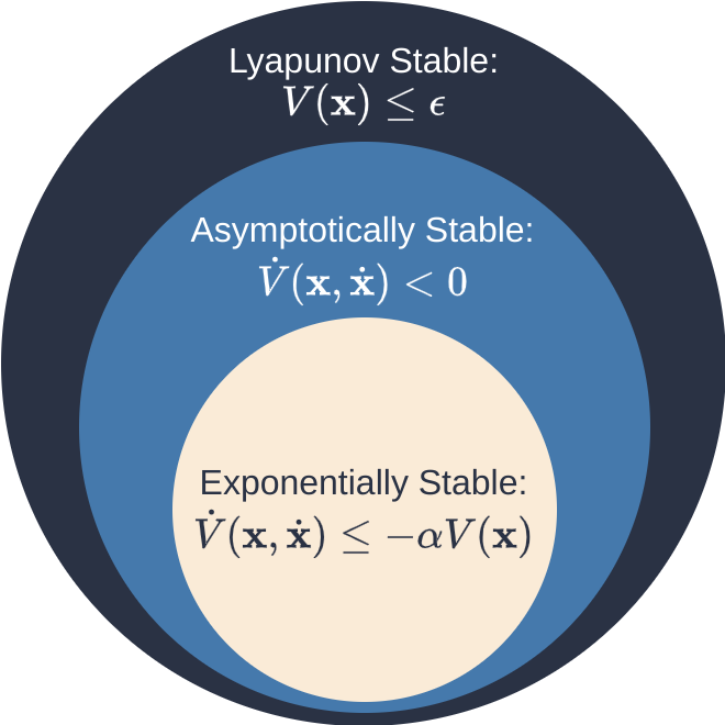
Every exponentially stable system is asymptotically stable, and every asymptotically stable system is Lyapunov stable.
A 3-Step Process
In a previous article, I showed a 3 step process for solving feedback control of linear systems. The exact same process applies here. If we have a position or configuration vector $\mathbf{x}\in\mathbb{R}^n$ then:
- Define the error from some desired configuration $\boldsymbol{\epsilon} = \mathbf{x}_d - \mathbf{x}$,
- Evaluate the time derivative $\dot{\boldsymbol{\epsilon}} = ~?$
- Choose the input that forces the error to decay: $\dot{\boldsymbol{\epsilon}} = -\mathbf{K}\boldsymbol{\epsilon}~\Longrightarrow~\boldsymbol{\epsilon}(t) = e^{-\mathbf{K}t}\boldsymbol{\epsilon}(0)$.
For the non-linear case, we need only make a slight modification:
- Define the error from some desired configuration $\boldsymbol{\epsilon} = \mathbf{x}_d - \mathbf{x}$,
- Formulate a Lyapunov function $V(\boldsymbol{\epsilon}) \ge 0 ~\forall\boldsymbol{\epsilon}$.
- Evaluate the time derivative $\dot{V}(\boldsymbol{\epsilon},\dot{\boldsymbol{\epsilon}}) = ~?$
- Choose the control input that forces the error to asymptotically decay $\dot{V}(\boldsymbol{\epsilon},\dot{\boldsymbol{\epsilon}}) \le 0$.
There are no rules or guidelines for choosing the Lyapunov candidate function, other than that it is positive. But as we saw from the pendulum example, an energy-like quantity is an excellent choice. It allows us to appeal to physics principles which gives intuitive results.
Another thing to consider is that energy is quadratic with respect to velocity, and in some cases, with respect to configuration as well. This is really nice because quadratic functions have a single, global minimum, and we can visualise the energy of 1D systems easily (see figure below). For example, a mass-spring-damper system has the energy:
\[E(x,\dot{x}) = \frac{1}{2}m\dot{x}^2 + \frac{1}{2}k(x-x_0)^2 \tag{15}\]where $x_0$ is the resting position. It is quadratic in both position (configuration), and velocity. In a more abstract sense, it contains the sum-of-squares $x^2,~\dot{x}^2$. So, the sum-of-squared errors is often the best choice for a Lyapunov candidate function.
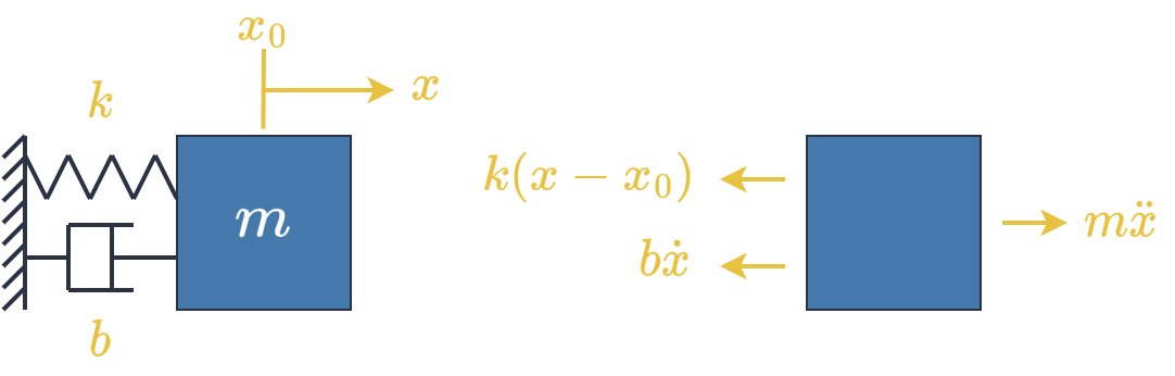
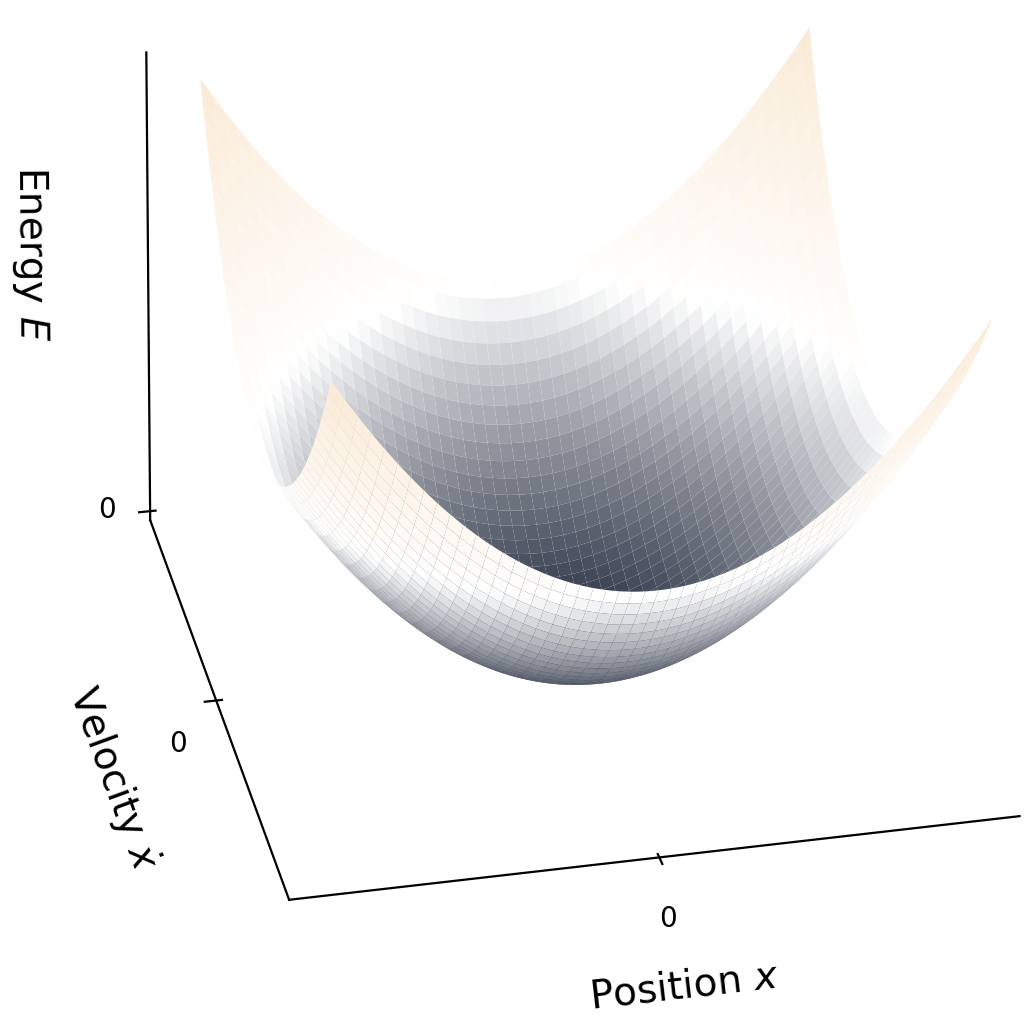
The energy in a mass-spring-damper system is quadratic with respect to both position, and velocity.
Quaternions
Quaternions are sophisticated mathematical objects that are used to represent orientation in 3D space. They are used in animation, videogames, aerospace, and robotics. In the latter two fields, orientation control is particularly important. Quaternions form a Lie group $\mathbb{H}$, and those which represent orientation are a subset of this $\mathbb{S}^3\subset\mathbb{H}$. Lie groups have specific rules for combining objects, which can make them highly nonlinear. In specific cases, Lyapunov stability is the most straightforward method for stability proofs.
A quaternion contains four elements, often represented as a scalar part and vector part:
\[\boldsymbol{v} = \begin{bmatrix} \eta \\ \boldsymbol{\varepsilon} \end{bmatrix} \in\mathbb{S}^3 \subset \mathbb{H} \tag{16}\]which, in the case of orientation, we have:
- $\eta = \cos(\tfrac{1}{2}\alpha) = [0, 1]$ as the scalar,
- $\boldsymbol{\varepsilon} = \sin(\tfrac{1}{2}\alpha)\hat{\mathbf{a}} \in\mathbb{R}^3$ as the vector,
- $\alpha = [0,2\pi]$ is the angle of rotation, and
- $\hat{\mathbf{a}}\in\mathbb{R}^3 ~:~ \hat{\mathbf{a}}^T\hat{\mathbf{a}} = 1$ is the axis of rotation.
The unit norm condition (the Euler-Rodrigues parameters) is such that:
\[\eta^2 + \boldsymbol{\varepsilon}^T\boldsymbol{\varepsilon} = 1. \tag{17}\]Before we can formulate the feedback control problem, we will need several important properties to exploit.
Properties of Quaternions
Closure:
This is a fundamental property of Lie groups. When we combine 2 elements in a Lie group, we get a 3rd. For the quaternion, we follow a unique arithmetic for combining rotations together:
Identity:
This is the element of a group that results in no change. By multiplying a quaternion with the identity, we end up with the original quaternion. The identity of a quaternion contains zero in the vector component:
We can reverse engineer this to see that it equates to zero rotation: $\alpha = 2\cdot\arccos(1) =0$.
Inverse:
Applying the closure property to the inverse element of a Lie group leads to the identity. For quaternions, we negate the vector component, otherwise known as its conjugate:
Time Derivative:
Evaluating the time derivative for a quaternion involves appealing to L’Hopital’s rule, and the closure property. It’s a little complex, so the proof is outside the scope of this article. Simply stated, the time derivative is:
where $\boldsymbol{\omega}\in\mathbb{R}^3$ is the angular velocity vector (rad/s), and:
\[S(\boldsymbol{\omega}) = \begin{bmatrix} \phantom{-}0 & -\omega_z & \phantom{-}\omega_y \\ \phantom{-}\omega_z & \phantom{-}0 & -\omega_x \\ -\omega_y & \phantom{-}\omega_x & 0 \end{bmatrix} \tag{22}\]is a skew-symmetric matrix.
Quaternion Error:
Now we can give a proper definition to the quaternion error. We apply the closure and inverse between the desired and actual:
We can see that if $\boldsymbol{v} = \boldsymbol{v}_d$ then this leads to the identity.
An analogy is addition over real vectors $\mathbf{x}\in\mathbb{R}^n$ which also form a Lie group. To define error, we would use addition (closure) with subtraction (inverse):
\[\boldsymbol{\epsilon} = \mathbf{x}_d + (-\mathbf{x}). \tag{24}\]When $\mathbf{x} = \mathbf{x}_d$, we get the identity element (zero):
\[\mathbf{x} = \mathbf{x}_d~\longrightarrow~\boldsymbol{\epsilon} = \mathbf{0}. \tag{25}\]Feedback Control
This proof for quaternion feedback control is from a research paper you can find online2. To replicate it, we will follow my 3 step process. First, we define a Lyapunov candidate function as the sum-of-square errors:
\[\begin{align} V(\boldsymbol{e}) &= \left(\eta_d - \eta\right)^2 + \left(\boldsymbol{\varepsilon}_d - \boldsymbol{\varepsilon}\right)^T\left(\boldsymbol{\varepsilon}_d - \boldsymbol{\varepsilon}\right) \tag{26a} \\ &= 2 - 2\left(\eta_d\eta +\boldsymbol{\varepsilon}_d^T\boldsymbol{\varepsilon}\right) \ge 0 \tag{26b} \end{align}\]Notice that with sufficient algebraic manipulation this reduces to the scalar component of the quaternion error.
Second, we take the time derivative, substituting in the quaternion velocity equation to obtain:
\[\dot{V}(\boldsymbol{e},\dot{\boldsymbol{e}}) = -2\dot{\eta}_e = \left(\boldsymbol{\omega}_d - \boldsymbol{\omega}\right)^T\boldsymbol{\varepsilon}_e. \tag{27}\]Third, we choose our control input $\boldsymbol{\omega}$ so that this will asymptotically decay:
\[\boldsymbol{\omega} \triangleq \boldsymbol{\omega}_d + \mathbf{K}\boldsymbol{\varepsilon}_e \tag{28}\]where $\mathbf{K}\in\mathbb{R}^{3\times 3}$ is a gain matrix. If we substitute this in, then:
\[\dot{V}(\boldsymbol{e},\dot{\boldsymbol{e}}) = -\boldsymbol{\varepsilon}_e^T\mathbf{K}\boldsymbol{\varepsilon}_e < 0 ~\forall \boldsymbol{\varepsilon}_e\ne\mathbf{0}. \tag{29}\]If we design $\mathbf{K}$ so that it is positive definite (symmetric, with positive, real, eigenvalues) then this is guaranteed to be monotonically non-increasing. Thus the feedback control law is asymptotically stable. An easy choice for $\mathbf{K}$ is to make it a diagonal matrix.
The animation below shows a robot using quaternion feedback control. It is a standard part of RobotLibrary.
Quaternion feedback used to control the orientation.
A very important note here: both $\boldsymbol{v}$ and $-\boldsymbol{v}$ represent the same orientation with quaternions! This can cause your robot to suddenly spin 360$^\circ$ toward the desired orientation. Since quaternions can be represented as a 4D vector, we can check if they are point in the same direction using the dot product. If $\boldsymbol{v}_d \cdot \boldsymbol{v} < 0$, then simply use $-\boldsymbol{\varepsilon}_e$ in the feedback control law to spin the opposite direction.
-
Lyapunov, A. M. (1892). The General Problem of the Stability of Motion. Kharkov Mathematical Society. Originally in Russian. English translation by A.T. Fuller, London: Taylor & Francis, 1992. ↩
-
Yuan, J. (1988). Closed-loop manipulator control using quaternion feedback. IEEE Journal on Robotics and Automation, 4(4):434–440. ↩