Linear Feedback Control in 3 Easy Steps
In this post I reveal my approach to solving (almost) all control problems. The first is to start from a physical principle. We are all bound by the laws of physics, so using physics principles to formulate control laws leads to elegant solutions. The second is a simple 3-step process to ensure stability of linear systems. I apply this to first order, and second order systems. At the end I show how it can be applied to robot arm control.
🧭 Navigation
- Thinking Like a Physicist
- A 3-Step Process
- First Order Systems
- Second Order Systems
- A Real Control Problem?
- References
Thinking Like a Physicist
There are many natural phenomena that exhibit stable behaviour. Or at the very least, their dynamic behaviour remains consistent over time. For example, the temperature of a hot cup of coffee will eventually cool until it equalises around room temperature:

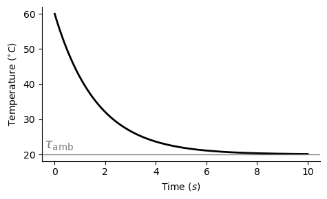
The temperature of a cup of coffee will decay exponentially toward the ambient temperature. (That is actually a photo of a coffee I made when working as a barista in 2007!)
The rate of change in the temperature of the coffee $\frac{d\tau}{dt}= \dot{\tau}(t)$ (K/s) is proportional to the difference between its current temperature $\tau(t)$ (K) and the ambient temperature $\tau_{amb.}$ (K):
\[\dot{\tau}(t) = k\cdot\left(\tau_{amb.} - \tau(t)\right) \tag{1}\]where $k\in\mathbb{R}^+$ (1/s) is some (positive) constant.
This is an ordinary differential equation, so the solution for $\tau(t)$ is an exponential:
\[\tau(t) = e^{-kt}\tau(0) + (1 - e^{-kt})\tau_{amb.} \tag{2}\]Equation (2) s a little cumbersome. Let’s instead consider the difference between the ambient temperature and that of the coffee:
\[\begin{align} \epsilon(t) &= \tau_{amb.} - \tau(t) \tag{3a}\\ \dot{\epsilon}(t) &= -\dot{\tau} \tag{3b} \\ &= -k\cdot\underbrace{\left(\tau_{amb}. - \tau(t)\right)}_{\epsilon(t)} \tag{3c} \end{align}\]The solution is a much simpler exponential equation of the form:
\[\therefore \epsilon(t) = e^{-kt}\epsilon(0). \tag{4}\]The difference between the environment and the cup of coffee decays to zero over time; whether it is hotter or colder.
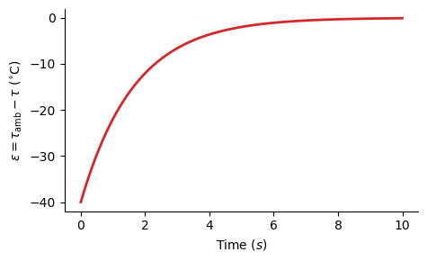
The difference in temperature asymptotically approaches zero.
All autonomous systems are bound by the laws of physics. By framing control problems with respect to natural laws and observed phenomena, we not only obtain elegant solutions, but equations that are easy to interpret.
A 3-Step Process
As with the heat decay of coffee, the objective of control is to force the difference between a desired system state and and the actual system state, i.e. the error, to exponentially decay. This can be solved using a straightforward 3-step process:
- Define the position error $\boldsymbol{\epsilon} = \mathbf{x}_d - \mathbf{x}$
- Evaluate how the error evolves with time $\dot{\boldsymbol{\epsilon}} = ~?$
- Design the control input to force the errors to decay: $\dot{\boldsymbol{\epsilon}} = -\mathbf{K}\boldsymbol{\epsilon} \Longrightarrow \boldsymbol{\epsilon} = e^{-\mathbf{K}t}\boldsymbol{\epsilon}_0$
The most complicated step is the 3rd, as the form of the control equation depends on the structure of the system.
First Order Systems
Consider a linear, control affine system:
\[\dot{\mathbf{x}} = \mathbf{Ax + Bu} \tag{5}\]where:
- $\mathbf{x}\in\mathbb{R}^m$ is the configuration,
- $\dot{\mathbf{x}}\in\mathbb{R}^m$ is its time derivative,
- $\mathbf{A}\in\mathbb{R}^{m\times m}$ is the state transition matrix,
- $\mathbf{B}\in\mathbb{R}^{m\times n}$ is the control matrix, and
- $\mathbf{u}\in\mathbb{R}^n$ is the control input.
Suppose now we have a desired state $\mathbf{x}_d,\dot{\mathbf{x}}_d\in\mathbb{R}^m$ (typically given by a trajectory), and we want to solve for the control input $\mathbf{u}$ such that $\mathbf{x}\to\mathbf{x}_d$ . Following the 3-step process we:
1 Denote the error from the desired configuration:
\[\boldsymbol{\epsilon} = \mathbf{x}_d - \mathbf{x}. \tag{6}\]2 Evaluate the time derivative:
\[\begin{align} \dot{\boldsymbol{\epsilon}} &= \dot{\mathbf{x}}_d -\dot{\mathbf{x}} \tag{7a}\\ &= \dot{\mathbf{x}}_d - \mathbf{Ax - Bu}. \tag{7b} \end{align}\]Now we need to determine the control input $\mathbf{u}$ that forces the error derivative to be (negatively) proportional to itself:
\[\dot{\boldsymbol{\epsilon}} = -\mathbf{K}\boldsymbol{\epsilon} \quad\Longrightarrow \quad \boldsymbol{\epsilon} = e^{-\mathbf{K}t}\boldsymbol{\epsilon}_0 \quad \Longrightarrow \quad \lim_{t\to\infty} \boldsymbol{\epsilon}(t) = \mathbf{0} \tag{8}\]where $\mathbf{K}\in\mathbb{R}^{m\times m}$ is a gain matrix. This will cause the error to decay to zero over time.
3 Equate the relationship we desire, and solve for the control input $\mathbf{u}$:
\[\begin{align} \overbrace{\dot{\mathbf{x}}_d - \mathbf{Ax} - \mathbf{Bu}}^{\dot{\boldsymbol{\epsilon}}} &= -\mathbf{K}\boldsymbol{\varepsilon} \tag{9a}\\ \mathbf{Bu} &= \dot{\mathbf{x}}_d + \mathbf{K}\boldsymbol{\epsilon} -\mathbf{Ax} \tag{9b}\\ \mathbf{u} &= \mathbf{B}^{\dagger}\left(\dot{\mathbf{x}}_d + \mathbf{K}\boldsymbol{\epsilon} - \mathbf{Ax}\right) \tag{9c} \end{align}\]where:
\[\mathbf{B}^{\dagger} = \begin{cases} \left(\mathbf{B}^T\mathbf{B}\right)^{-1}\mathbf{B}^T & \text{for } m > n \\ \mathbf{B}^{-1} & \text{for } m = n \\ \mathbf{B}^T\left(\mathbf{BB}^T\right)^{-1} & \text{for } m < n \end{cases} \tag{10}\]is the (pseudo)inverse of $\mathbf{B}$.
Equation (3d) is a scalar, so if the exponent is negative, the system will decay (i.e. stable). If it is positive, then it will grow (unstable). However, Eqn. (8) is a matrix exponential. The system is stable if the matrix $\mathbf{K}$ has positive eigenvalues (such that $-\mathbf{K}$ has negative eigenvalues). Why? That’s beyond the scope of this article…!
Second-Order Systems
The dynamics of many systems is naturally expressed & controlled at the acceleration or force level. The process for solving feedback control for second order system is the same.
1 Define the position error:
\[\boldsymbol{\epsilon} = \mathbf{x}_d - \mathbf{x} \tag{11}\]2 Evaluate the time derivatives:
\[\begin{align} \dot{\boldsymbol{\epsilon}} &= \dot{\mathbf{x}}_d - \dot{\mathbf{x}} \tag{12a} \\ \ddot{\boldsymbol{\epsilon}} &= \ddot{\mathbf{x}}_d - \ddot{\mathbf{x}}. \tag{12b} \end{align}\]To make the problem more tractable, we can express this second order system as an equivalent first order system and apply the same rules:
\[\begin{bmatrix} \dot{\boldsymbol{\epsilon}} \\ \ddot{\boldsymbol{\epsilon}} \end{bmatrix} = \begin{bmatrix} \mathbf{0} & \mathbf{I} \\ ? & ? \end{bmatrix} \begin{bmatrix} \boldsymbol{\epsilon} \\ \dot{\boldsymbol{\epsilon}} \end{bmatrix}. \tag{13}\]That is, we need to make the derivatives proportional to the anti-derivatives.
3 If we choose:
\[\ddot{\boldsymbol{\epsilon}} = -\mathbf{D}\dot{\boldsymbol{\epsilon}} - \mathbf{K}\boldsymbol{\epsilon} \tag{14}\]where:
- $\mathbf{D}\in\mathbb{R}^{m\times m}$ is a gain on the velocity error, and
- $\mathbf{K}\in\mathbb{R}^{m\times m}$ is a gain on the position error.
Now the system becomes:
\[\begin{bmatrix} \dot{\boldsymbol{\epsilon}} \\ \ddot{\boldsymbol{\epsilon}} \end{bmatrix} = \begin{bmatrix} \phantom{-}\mathbf{0} & \phantom{-}\mathbf{I} \\ -\mathbf{K} & -\mathbf{D} \end{bmatrix} \begin{bmatrix} \boldsymbol{\epsilon} \\ \dot{\boldsymbol{\epsilon}} \end{bmatrix}. \tag{15}\]We can choose values for $\mathbf{K}$ and $\mathbf{D}$ such that this composite matrix has negative eigenvalues.
By equating Eqn (12b) and (14) we can reverse engineer the “input” $\ddot{\mathbf{x}}$ as:
\[\ddot{\mathbf{x}} = \ddot{\mathbf{x}}_d + \mathbf{D}\dot{\boldsymbol{\epsilon}} + \mathbf{K}\boldsymbol{\epsilon}. \tag{16}\]Note the contribution of the 3 terms to the overall control equation:
- Feedforward acceleration $\ddot{\mathbf{x}}_d$,
- Velocity error feedback $\mathbf{D}\dot{\boldsymbol{\epsilon}}$, and
- Position error feedback $\mathbf{K}\boldsymbol{\epsilon}$.
A Real Control Problem?
With some abuse of notation, I am going to denote the position & orientation of the endpoint of a robot arm as:
\[\mathbf{x} = \mathbf{f}(\mathbf{q}) : \mathbb{R}^n\mapsto\mathbb{R}^m. \tag{17}\]This is known as forward kinematics. That is, given some joint configuration $\mathbf{q}\in\mathbb{R}^n$ we can compute the endpoint pose $\mathbf{x}\in\mathbb{R}^m$.
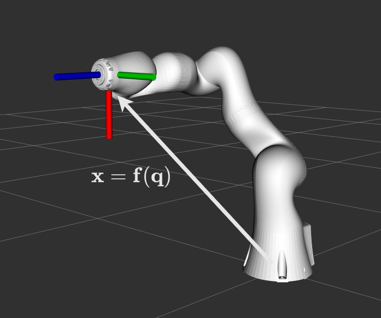
Forward kinematics is the method of computing the endpoint pose of a chain given the joint positions.
We want the endpoint pose to converge on some desired value $\mathbf{x}_d$. To do this we follow the same 3 step process.
1 Define the error:
\[\boldsymbol{\epsilon} = \mathbf{x}_d - \mathbf{f}(\mathbf{q}). \tag{18}\]2 Differentiate with respect to time:
\(\dot{\boldsymbol{\epsilon}} = \dot{\mathbf{x}}_d - \underbrace{\left(\partial\mathbf{f}/\partial\mathbf{q}\right)}_{\mathbf{J}(\mathbf{q})}\dot{\mathbf{q}}. \tag{19}\) The Jacobian $\mathbf{J}(\mathbf{q})$ can be evaluated numerically from the forward kinematics1
3 Equate the error and solve for the joint velocity $\mathbf{\dot{q}}$:
\[\begin{align} \overbrace{\dot{\mathbf{x}}_d - \mathbf{J}\dot{\mathbf{q}}}^{\dot{\boldsymbol{\epsilon}}} &= -\mathbf{K}\boldsymbol{\epsilon} \tag{20a} \\ \mathbf{J}\dot{\mathbf{q}} &= \dot{\mathbf{x}}_d + \mathbf{K}\boldsymbol{\epsilon} \tag{20b} \\ \dot{\mathbf{q}} &= \mathbf{J}^{\dagger}\left(\dot{\mathbf{x}}_d + \mathbf{K}\boldsymbol{\epsilon}\right) \tag{20c} \end{align}\]where $\mathbf{J}^{\dagger}\in\mathbb{R}^{n\times m}$ is the (pseudo)inverse, as in Eqn. (10).
We can use this method to make the robot follow a trajectory in Cartesian space. This idea was first proposed by Whitney (1969)2.
![]()
The code for the animation is implemented using my ROS2 velocity control action server, which you can find here.