Hamiltonian Mechanics

In classical mechanics, the Lagrangian is defined as the difference between kinetic and potential energy. We use this to solve for the equations of motion for systems of rigid bodies. But what is its relationship to the conservation of energy, which states the sum of kinetic and potential is constant? In this article I show how to derive the Hamiltonian from the Lagrangian, i.e. the sum of kinetic and potential for rigid body systems. I then show how momentum is used in lieu of velocity to define phase space, and touch on its implications with respect to the Hamiltonian.

📄 Download a PDF version.

🧭 Navigation

• The Conservation of Energy
• Systems of Rigid Bodies
  • The Lagrangian
  • Deriving the Hamiltonian
• Momentum
  • What Newton Really Said
  • Re-Visiting the Lagrangian
  • Phase Space

The Conservation of Energy

One of the most important principles in physics is the conservation of energy. When an apple falls from a tree, it loses potential energy but gains kinetic energy. The total energy remains constant for all time (until it hits someone on the head).

A falling apple loses potential energy and gains kinetic energy as it falls.

We can use this principle to solve for the state of an object at any given time. If $x\in\mathbb{R}$ is its position, and $\dot{x}\in\mathbb{R}$ is its velocity, then at any 2 given points in time it must hold that:

\[\tfrac{1}{2}m\dot{x}_1^2 + mgx_1 = \tfrac{1}{2}m\dot{x}_2^2 + mgx_2. \tag{1}\]

in which $m\in\mathbb{R}^+$ is the mass (kg), and $g\in\mathbb{R}$ is gravitational acceleration. So, for example, given $x_1,~\dot{x}_1$ and $x_2$ we could determine the speed just before it hits the ground $\dot{x}_2$.

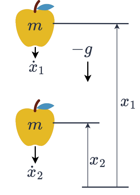
We can use conservation of energy to solve for state variables at different points in time.

In fact, we can use the conservation of energy to derive Newton’s second law: \(\begin{align} \frac{d}{dt}\left(\tfrac{1}{2}m\dot{x}^2 + mgx\right) &= 0 \tag{2a} \\ m\dot{x}\ddot{x} + mg\dot{x} &= 0 \tag{2b} \\ m\ddot{x} &= -mg. \tag{2c} \end{align}\)

🔝 Back to top.

Systems of Rigid Bodies

The Lagrangian

Lagrangian mechanics extends Newton’s second law and enables us to solve the dynamic equations of motion for systems of rigid bodies. Suppose $\mathbf{q}\in\mathbb{R}^n$ is the configuration vector, and $\dot{\mathbf{q}}\in\mathbb{R}^n$ is the velocity vector. Hamilton noted that we could first define a functional as the difference between kinetic energy (kinetic energy is now configuration dependent) and potential energy.¹

\[\mathcal{L}(\mathbf{q},\dot{\mathbf{q}}) = \mathcal{K}(\mathbf{q},\dot{\mathbf{q}}) - \mathcal{P}(\mathbf{q}) : \mathbb{R}^{n}\times\mathbb{R}^n\mapsto\mathbb{R}. \tag{3}\]

This is known as the Lagrangian. Then, from the calculus of variations, this function is an extremum (maximum or minimum) when its variation is zero $\delta\mathcal{L} = 0$. This leads to the Euler-Lagrange equation:

\[\frac{d}{dt}\left(\frac{\partial\mathcal{L}}{\partial\dot{\mathbf{q}}}\right) - \frac{\partial\mathcal{L}}{\partial\mathbf{q}} = \mathbf{0}. \tag{4}\]

Using Hamilton’s definition Eqn. (3) gives Lagrange’s equations of motion.²

This is strange, though, right? From the conservation of energy we would expect the sum of kinetic and potential, yet the Lagrangian requires the difference between the two. What is the relationship between them?

🔝 Back to top.

Deriving the Hamiltonian

If we were to take the time derivative of Eqn. (3) then we would obtain:

\[\begin{align} \dot{\mathcal{L}} &= \dot{\mathbf{q}}^T\frac{\partial\mathcal{L}}{\partial\mathbf{q}} + \ddot{\mathbf{q}}^T\frac{\partial\mathcal{L}}{\partial\dot{\mathbf{q}}} \tag{5a} \\ &= \underbrace{\dot{\mathbf{q}}^T\frac{d}{dt}\left(\frac{\partial\mathcal{L}}{\partial\dot{\mathbf{q}}}\right) + \ddot{\mathbf{q}}^T\frac{\partial\mathcal{L}}{\partial\dot{\mathbf{q}}}}_{\frac{d}{dt}\left(\frac{\partial\mathcal{L}}{\partial\dot{\mathbf{q}}}\right)} \tag{5b} \end{align}\]

But now we can integrate with respect to time to get back an expression containing the original Lagrangian:

\[\mathcal{L}(\mathbf{q},\dot{\mathbf{q}}) = \dot{\mathbf{q}}^T\frac{\partial\mathcal{L}}{\partial\dot{\mathbf{q}}} + \text{const.} \tag{6}\]

Notice how the constant appears due to the rules of integral calculus. Now we can simply re-arrange and define the Hamiltonian:

\[\mathcal{H}(\mathbf{q},\dot{\mathbf{q}}) = \dot{\mathbf{q}}^T\frac{\partial\mathcal{L}}{\partial\dot{\mathbf{q}}} - \mathcal{L}(\mathbf{q},\dot{\mathbf{q}}) \tag{7}\]

which is constant in a conservative system.

In a rigid body system the kinetic energy is:

\[\mathcal{K}=\frac{1}{2}\dot{\mathbf{q}}^T\mathbf{M}(\mathbf{q})\dot{\mathbf{q}} \tag{8}\]

where $\mathbf{M}(\mathbf{q})=\mathbf{M}(\mathbf{q})^T\in\mathbb{R}^{n\times n}$ is the generalised inertia matrix. By putting this back in to Eqn. (7) we now obtain a much more familiar form:

\[\mathcal{H}(\mathbf{q},\dot{\mathbf{q}}) = \mathcal{K}(\mathbf{q},\dot{\mathbf{q}}) + \mathcal{P}(\mathbf{q}). \tag{9}\]

🔝 Back to top.

Momentum

What Newton Really Said

Newton didn’t actually express his second law as “force = mass x acceleration”, as people often recite. What he said was:

“Lex II: Mutationem motus proportionalem esse vi motrici impressae, et fieri secundum lineam rectam qua vis illa imprimitur.” ³

or translated to English:

“Law II: The change of motion is proportional to the motive force impressed; and is made in the direction of the straight line in which that force is impressed.”

Here, “motion” is better conceptualised as “momentum”, i.e. the product of mass and velocity. The time derivative of momentum is equal to the forces applied. In a 1D system we would write:

\[p = m\dot{x}~\Longrightarrow~ f = \frac{dp}{dt} = m\ddot{x}. \tag{10}\]

For a system of rigid bodies, we denote the generalised momentum as:

\[\mathbf{p} \triangleq \mathbf{M}(\mathbf{q})\dot{\mathbf{q}} = \frac{\partial\mathcal{L}}{\partial\dot{\mathbf{q}}} \tag{11}\]

which, from Eqn. (3) and Eqn. (8), is the partial derivative of the Lagrangian with respect to velocity.

🔝 Back to top.

Re-Visiting the Lagrangian

If we re-arrange Eqn. (4) and substitute in Eqn. (11) we obtain:

\[\begin{align} \frac{d}{dt}\left(\frac{\partial\mathcal{L}}{\partial\dot{\mathbf{q}}}\right) &= \frac{\partial\mathcal{L}}{\partial\mathbf{q}} \tag{12a}\\ \dot{\mathbf{p}} &= \frac{\partial\mathcal{K}}{\partial\mathbf{q}} - \frac{\partial\mathcal{P}}{\partial\mathbf{q}} \tag{12b} \\ \mathbf{M}\ddot{\mathbf{q}} + \dot{\mathbf{M}}\dot{\mathbf{q}} &= \frac{1}{2}\dot{\mathbf{q}}^T\frac{\partial\mathbf{M}}{\partial\mathbf{q}}\dot{\mathbf{q}} - \mathbf{g}. \tag{12c} \end{align}\]

where $\mathbf{g} = \frac{\partial \mathcal{P}}{\partial\mathbf{q}}$ it the generalised gravitational force vector.

On the left hand side of Eqn. (12c) we have the familiar mass by acceleration $\mathbf{M}\ddot{\mathbf{q}}$. But a new term appears, $\dot{\mathbf{M}}\dot{\mathbf{q}}$. This is because, in a system of rigid bodies, the distribution of mass can also change over time. Then, on the right hand side, we see the effect of gravity $\mathbf{g}$, but also the forces due to a configuration change.

So Lagrange’s equations of motion are just a generalisation of Newton’s second law. The time derivative of momentum is equal to the force applied. But it accounts for the change in configuration, and the subsequent change in the distribution of mass.

If we consider the case where $\dot{\mathbf{q}} = \mathbf{0}$, then Eqn. (12c) reduces to a much more familiar form:

\[\mathbf{M}\ddot{\mathbf{q}} = -\mathbf{g}. \tag{13}\]

🔝 Back to top.

Phase Space

If we have the system configuration $\mathbf{q}$ and its time derivative $\dot{\mathbf{q}}$, then we have all the information we need to reconstruct its equations of motion under its own impetus.⁴ The concatenation of the two gives the state space vector:

\[\mathbf{x} = \begin{bmatrix} \mathbf{q} \\ \dot{\mathbf{q}} \end{bmatrix} ~\longrightarrow ~ \dot{\mathbf{x}} = \begin{bmatrix} \dot{\mathbf{q}} \\ \ddot{\mathbf{q}} \end{bmatrix}. \tag{14}\]

We could instead consider phase space as configuration and momentum:

\[\mathbf{y} = \begin{bmatrix} \mathbf{q} \\ \mathbf{p}\end{bmatrix}. \tag{15}\]

Now using Eqn. (7) & (11) we can express the Hamiltonian as a function of momentum:

\[\mathcal{H}(\mathbf{p},\mathbf{q}) = \dot{\mathbf{q}}^T\mathbf{p} - \mathcal{L}(\mathbf{q},\dot{\mathbf{q}}). \tag{16}\]

We can actually use this to generate the dynamic equations of motion. The trick is to treat $\mathbf{p}$ and $\mathbf{q}$ as independent variables. First, we can easily recover the velocity from Eqn. (16) by taking the partial derivative with respect to momentum:

\[\dot{\mathbf{q}} = \frac{\partial\mathcal{H}}{\partial\mathbf{p}}. \tag{17}\]

Then from Eqn. (12) & (16) we can get the time derivative of momentum:

\[\begin{align} \dot{\mathbf{p}} = \frac{d}{dt}\left(\frac{\partial\mathcal{L}}{\partial\dot{\mathbf{q}}}\right) = \frac{\partial\mathcal{L}}{\partial\mathbf{q}} = -\frac{\partial\mathcal{H}}{\partial\mathbf{q}}. \tag{18} \end{align}\]

This is interesting because the Hamiltonian is 1 dimensional, and this means we can conceptualise it as an energy surface. This also means the time derivative of the phase space is a vector on this surface:

\[\dot{\mathbf{y}} = \begin{bmatrix} \dot{\mathbf{q}} \\ \dot{\mathbf{p}} \end{bmatrix} = \begin{bmatrix} \phantom{-}\partial\mathcal{H}/\partial\mathbf{p} \\ -\partial\mathcal{H}/\partial\mathbf{q} \end{bmatrix}. \tag{19}\]

A conservative system $\dot{H} = 0$ will follow a single contour line along this surface, i.e. a fixed level set.

A conservative system will remain on a single contour line in the phase portrait.

🔝 Back to top.