Lagrangian Mechanics Is Just A Generalisation of Newtonian Mechanics

Lagrangian mechanics is a sophisticated method for deriving the equations of motion for a dynamic system. The key principle is that it minimises the difference between kinetic and potential energy, integrated across time. But why? In this article, I trace the derivation from Newton’s second principle, to Lagrange’s formulation, to Hamilton’s principle of least action. I show that Lagrangian mechanics is just a generalisation of Newton’s law, extended to multi-body systems.

📄 Download a PDF version.

🧭 Navigation

• Force or Energy?
• Lagrangian Mechanics
  • Lagrange’s Generalisation
  • What Does It All Mean?
• The Principle of Least Action

Force or Energy?

Between 1589 and 1592, Galileo Galilei supposedly dropped two objects of different masses from the Leaning Tower of Pisa to show that acceleration is independent of mass.

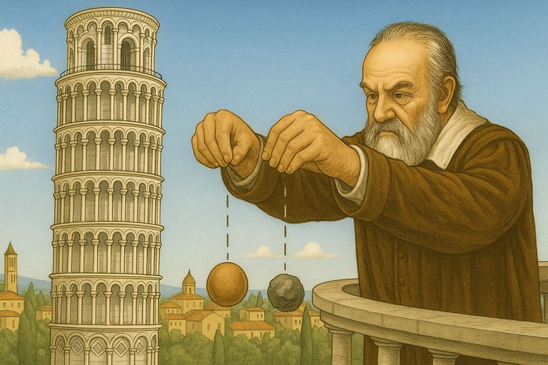
Galileo demonstrated that acceleration is independent of mass by dropping two different objects from the Tower of Pisa.

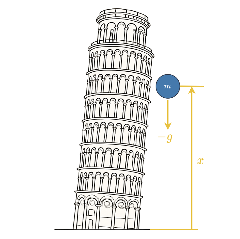
About 100 years later, in 1687, Sir Isaac Newton published his laws of motion in the Principia Matematica¹. His second law of motion codified what Galileo had observed; that the acceleration due to gravity $\frac{d^2 x}{dt^2} = \ddot{x}$ is independent of mass. In light of Galileo’s experiment we would write the equation of motion for a falling object as:

\[m\ddot{x} = -mg ~\Longrightarrow~ \ddot{x} = -g \tag{1}\]

where:

• $m$ is the mass (kg), and
• $g$ is gravitational acceleration (m/s/s).

Assuming the object starts with zero velocity, we can compute its speed when it impacts the ground using integration:

\[\dot{x}_f = \int_{t_0}^{t_f} \ddot{x}~dt. \tag{2}\]

But there’s another way we could solve this problem. The potential energy of an object at any given height is:

\[\mathcal{P}(x) = mgx. \tag{3}\]

The gravitational potential energy in an object is a function of its height. This is converted to kinetic energy as it falls.

And when it hits the ground all of this potential energy is converted to kinetic energy:

\[\mathcal{K}(\dot{x}) = \frac{1}{2}m\dot{x}^2. \tag{4}\]

By equating the two we can solve:

\[\begin{align} \frac{1}{2}m\dot{x}_f^2 &= mgx_0 \tag{5a} \\ \dot{x}_f &= \sqrt{2 g x_0}. \tag{5b} \end{align}\]

So there are 2 ways to frame this problem that result in the same solution: force, or energy.

⬆️ Back to top.

Lagrangian Mechanics

Lagrange’s Generalisation

It is well established that forces in a potential field are the negative of the gradient:

\[\mathcal{P}(x) = mgx ~\Longrightarrow~ f_g = -\frac{d\mathcal{P}}{dx} = -mg. \tag{6}\]

But the dynamic forces $m\ddot{x}$ may also be expressed in terms of derivatives of kinetic energy. Specifically, we could re-write Newton’s second law as:

\[\underbrace{\frac{d}{dt}\left(\frac{d\mathcal{K}}{d\dot{x}}\right)}_{m\ddot{x}} = \underbrace{-\frac{d\mathcal{P}}{dx}\vphantom{\begin{bmatrix} a\\ b\end{bmatrix}}}_{-mg}. \tag{7}\]

Newton’s laws concern particles; individual, rigid bodies. But Lagrange’s genius was to generalise these principles to systems of rigid bodies². Now we consider the configuration for a rigid body system denoted by $\mathbf{q}\in\mathbb{R}^n$ (e.g., a vector of joint angles for a robot), and the associated velocities $\dot{\mathbf{q}}\in\mathbb{R}^n$.

If the energy in a closed system is conserved, then it follows that an infinitesimal change in the kinetic energy must equal an infinitesimal change in potential energy:

\[\delta\mathcal{K} = \delta\mathcal{P}. \tag{8}\]

Three things to keep in mind here:

1. We don’t consider the signs here, as you might expect from Eqn. (7); it will be resolved implicitly.
2. Lagrange actually appealed to d’Alembert’s principle, but I think this approach is a little more straightforward.
3. Kinetic energy is now configuration dependent: $\mathcal{K}(\mathbf{q},\dot{\mathbf{q}})$.

Taking the variation, we consider the effect of infinitesimal changes in configuration $\delta\mathbf{q}$ and velocity $\delta\dot{\mathbf{q}}$ on energy balance:

\[\delta\mathbf{q}^T\frac{\partial\mathcal{K}}{\partial\mathbf{q}} + \delta\dot{\mathbf{q}}^T\frac{\partial\mathcal{K}}{\partial\dot{\mathbf{q}}} = \delta\mathbf{q}^T\frac{\partial\mathcal{P}}{\partial\mathbf{q}}. \tag{9}\]

Then we can use integration by parts to eliminate $\delta\dot{\mathbf{q}}$:

\[\delta\dot{\mathbf{q}}^T\frac{\partial\mathcal{K}}{\partial\dot{\mathbf{q}}} = -\delta\mathbf{q}^T\frac{d}{dt}\left(\frac{\partial \mathcal{K}}{\partial\dot{\mathbf{q}}}\right). \tag{10}\]

Now putting Eqn. (10) back in to Eqn (9) we obtain:

\[\begin{align} \delta\mathbf{q}^T\left(\frac{\partial\mathcal{K}}{\partial\mathbf{q}} -\frac{d}{dt}\left(\frac{\partial \mathcal{K}}{\partial\dot{\mathbf{q}}}\right)\right) &= \delta\mathbf{q}^T\frac{\partial\mathcal{P}}{\partial\mathbf{q}} \tag{11a} \\ \frac{d}{dt}\left(\frac{\partial \mathcal{K}}{\partial\dot{\mathbf{q}}}\right) - \frac{\partial\mathcal{K}}{\partial\mathbf{q}} &= -\frac{\partial P}{\partial\mathbf{q}}. \tag{11b} \end{align}\]

Equation (11a) is d’Alemberts principle. It is the projection of a virtual displacement $\delta\mathbf{q}$ on to the forces acting on the system, which should sum to zero.³ More importantly, Eqn. (11b) is Lagrange’s equations for the dynamics of a rigid body system. Note its structural similarity to (a generalisation of) Eqn. (7).

⬆️ Back to top.

What Does It All Mean?

What is Eqn. (11b) telling us?

Firstly, Newton didn’t state his second law as “force equals mass times acceleration”, as often recited. What he wrote was:

“Lex II: Mutationem motus proportionalem esse vi motrici impressae, et fieri secundum lineam rectam qua vis illa imprimitur.” ¹

or in English:

“Law II: The change of motion is proportional to the motive force impressed; and is made in the direction of the straight line in which that force is impressed.”

In modern parlance we would say that force is equal to the time derivative of momentum. For a system of rigid bodies, we would denote its generalised inertia matrix as $\mathbf{M}(\mathbf{q}) = \mathbf{M}(\mathbf{q})^T\in\mathbb{R}^{n\times n}$. Then its kinetic energy is:

\[\mathcal{K}(\mathbf{q},\dot{\mathbf{q}}) = \frac{1}{2}\dot{\mathbf{q}}^T\mathbf{M}(\mathbf{q})\dot{\mathbf{q}} \tag{12}\]

and the momentum:

\[\mathbf{p} = \mathbf{M}(\mathbf{q})\dot{\mathbf{q}} = \frac{\partial\mathcal{K}}{\partial\dot{\mathbf{q}}}. \tag{13}\]

So:

• $\frac{d}{dt}\left(\frac{\partial\mathcal{K}}{\partial\dot{\mathbf{q}}}\right) = \frac{d\mathbf{p}}{dt}$ is the change in momentum,
• $\frac{\partial\mathcal{K}}{\partial\mathbf{q}}$ are internal forces from a configuration change, and
• These are both induced by the potential field through $-\frac{\partial\mathcal{P}}{\partial\mathbf{q}}$.

⬆️ Back to top.

The Principle of Least Action

There was a different thread running through history at the same time. In 1744 Pierre-Louis Moreau de Maupertuis philosophised that:

“…in all changes that happen in nature, the amount of action is as small as possible.” ⁴

He would later denote this as the integral of momentum over distance, which is twice the kinetic energy across time:

\[A = \int m\dot{x} ~dx = \int m\dot{x}^2~dt. \tag{14}\]

This didn’t pan out, as evinced by history. Sir William Rowan Hamilton would propose its canonical form still used in classical mechanics today⁵. He observed that Lagrange’s equations of motion, Eqn. (11b), may be first be written as the functional:

\[\mathcal{L}(\mathbf{q},\dot{\mathbf{q}}) = \mathcal{K}(\mathbf{q},\dot{\mathbf{q}}) - \mathcal{P}(\mathbf{q}) ~:~ \mathbb{R}^{n}\times\mathbb{R}^n\mapsto\mathbb{R} \tag{15}\]

This is, unsurprisingly, referred to as the Lagrangian. Then, via the calculus of variations we obtain the (surprise!) Euler-Lagrange equation:

\[\frac{d}{dt}\left(\frac{\partial\mathcal{L}}{\partial\mathbf{\dot{q}}}\right) - \frac{\partial\mathcal{L}}{\partial\mathbf{q}} = \mathbf{0}. \tag{16}\]

This is equivalent to (11b). Reverse-engineering this, the action is defined as:

\[A = \int \underbrace{\mathcal{K}(\mathbf{q},\dot{\mathbf{q}}) - \mathcal{P}(\mathbf{q})\vphantom{\begin{matrix} a \\ b \end{matrix}}}_{\mathcal{L}(\mathbf{q},\dot{\mathbf{q}})}~dt \tag{17}\]

which has the SI units of joule-seconds. It follows that, for a conservative system, the equations of motion are an extremum of the action:

\[\delta A = \int \delta\mathcal{L}~dt = 0 ~\Longrightarrow~\delta L = 0 \tag{18}\]

whose solution is (16). The second variation, with respect to $\dot{\mathbf{q}}$, is:

\[\frac{\partial^2\mathcal{L}}{\partial\dot{\mathbf{q}}^2} = \mathbf{M}(\mathbf{q}) \succ 0. \tag{19}\]

The inertia matrix is positive definite, such that kinetic energy is always positive.⁶ Hence Eqn. (16), (11b) is a minimum of action.

Newton’s law is about the instantaneous balance of forces. Equation (17) is metric across time. That is, the trajectory that a system of rigid bodies will follow through a potential field will minimise the difference between all the forces acting on it.