Orientation Control With Angle-Axis Representation

In this article I provide some basic definitions and proofs of identities for rotation matrices $\mathbf{R}\in\mathbb{SO}(3)$. I show that a rotation matrix can be represented as a matrix exponential. From this, Rodrigues’ formula follows which expresses the matrix in terms of the angle and axis of rotation. I then show how to reverse this formula to obtain the angle and axis from an arbitrary rotation matrix. Then using the exponential form, and the angle-axis, I derive a control law for the angular velocity to perform feedback control on orientation error.

📄 Download a PDF version.

🧭 Navigation

• Euler’s Rotation Theorem
• Time Derivative & Exponential
• Angle & Axis from a Rotation Matrix
• Orientation Feedback Control

Euler’s Rotation Theorem

Euler’s rotation theorem states that any change in orientation of a rigid body can be described by:

• A single rotation $\alpha$ (rad),
• About an axis $\hat{\mathbf{a}}\in\mathbb{R}^3$ where $\hat{\mathbf{a}}$ is a unit vector such that $|\hat{\mathbf{a}}|^2 = \hat{\mathbf{a}}^T\hat{\mathbf{a}} = 1$.

The 3 combined rotations in the illustration below can be reduced to a single rotation about a single axis:

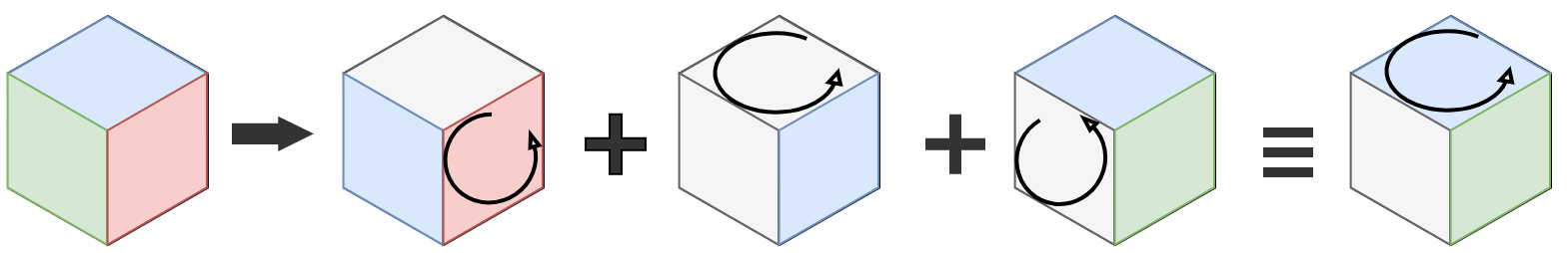
Any number of combined rotations can be expressed as a single rotation about a single axis.

Any transformation of a vector $\mathbf{v}\in\mathbb{R}^n\to\mathbf{u}\in\mathbb{R}^n$ that preserves its length can be expressed with a product involving a rotation matrix:

\[\mathbf{u} = \mathbf{Rv}. \tag{1}\]

This matrix belongs to the Special Orthogonal group:

\[\mathbb{SO}(n) = \Big\{\mathbf{R}\in\mathbb{R}^{n\times n} ~\Big|~ \mathbf{RR}^T = \mathbf{I}~,~ det(\mathbf{R}) = 1\Big\} \tag{2}\]

Given an arbitrary rotation matrix $\mathbf{R}\in\mathbb{SO}(3)$ we may be interested in finding the angle and axis of rotation. To do this, we need to define some other properties of $\mathbb{SO}(3)$ that we can exploit.

⬆️ Back to top.

Time Derivative & Exponential

If we take the time derivative of Eqn. (1), and assuming $\dot{\mathbf{v}} = \mathbf{0}$, then we arrive at:

\[\dot{\mathbf{u}} = \dot{\mathbf{R}}\mathbf{v}. \tag{3}\]

But in 3D, the time derivative of a vector is given by the cross product with the instantaneous angular velocity $\boldsymbol{\omega}\in\mathbb{R}^3$ (rad/s):

\[\mathbf{\dot{u}} = \boldsymbol{\omega}\times\mathbf{u} = S(\boldsymbol{\omega})\mathbf{u} \tag{4}\]

where $S(\cdot)$ is the skew-symmetric matrix operator:

\[S(\boldsymbol{\omega}) = \begin{bmatrix} \phantom{-}0 & -\omega_z & \phantom{-}\omega_y \\ \phantom{-}\omega_y & \phantom{-}0 & -\omega_x \\ -\omega_y & \phantom{-}\omega_x & \phantom{-}0 \end{bmatrix} \in\mathfrak{so}(3). \tag{5}\]

This is also the Lie algebra of $\mathbb{SO}(3)$. By equating Eqn. (3) with Eqn. (4), and substituting in Eqn. (1) we can see that the time derivative of the rotation matrix is “proportional” to itself:

\[\mathbf{\dot{R}} = S(\boldsymbol{\omega})\mathbf{R} ~\Longrightarrow \mathbf{R}(\mathrm{t}) = e^{S(\boldsymbol{\omega})\mathrm{t}}\mathbf{R}(0) \tag{6}\]

This is a first-order differential equation whose solution is a (matrix) exponential. But the integral of the angular velocity is simply the angle-axis vector at any given point in time:

\(\int_0^t \boldsymbol{\omega}~dt = \boldsymbol{\omega}t + const. = \alpha\cdot\hat{\mathbf{a}} = \mathbf{a}. \tag{7}\) (where $const. = 0$).

Assuming we start from zero rotation $(\mathbf{R}(0) = \mathbf{I})$, then the rotation matrix is equivalent to a matrix exponential containing the angle-axis:

\[\mathbf{R} = e^{S(\mathbf{a})}\in\mathbb{SO}(3). \tag{8}\]

From the definition of the exponential:

\[e^{S(\mathbf{a})} = \sum_{k=0}^\infty \frac{\alpha^{k}}{\mathrm{k!}}S(\hat{\mathbf{a}})^{k} \tag{9}\]

we can reduce Eqn. (8) to Rodrigues’ formula which features the angle and axis as separate parameters:

\[\mathbf{R}(\alpha,\hat{\mathbf{a}}) = \mathbf{I} + \sin(\alpha)S(\hat{\mathbf{a}}) + (1-\cos(\alpha))S(\hat{\mathbf{a}})^2. \tag{10}\]

⬆️ Back to top.

Angle & Axis from Rotation Matrix

Rodrigues’ formula, Eqn. (10), contains 3 matrices with a particular structure to their respective diagonal elements. If we take the trace (sum of diagonal elements) we can see that:

• $trace(\mathbf{I}) = 3$,
• $trace\left(S(\hat{\mathbf{a}})\right) = 0$, and
• $trace\left(S(\hat{\mathbf{a}})\right)^2 = -2$ since $|\hat{\mathbf{a}}| = 1.$

Hence the trace of a rotation matrix must be:

\[\begin{align} trace(\mathbf{R}) &= 3 - 2\cdot(1 - \cos(\alpha)) \tag{11a} \\ &= 1 + 2\cdot\cos(\alpha). \tag{11b} \end{align}\]

We can re-arrange this to solve for the angle of rotation:

\[\alpha = \cos^{-1}\left(\frac{trace(\mathbf{R}) - 1}{2}\right). \tag{12}\]

If the angle of rotation is zero $\alpha = 0$, then the axis of rotation is arbitrary since $0\cdot\hat{\mathbf{a}} = \mathbf{0}$.

The axis for a rotation matrix does not change $\mathbf{R}\hat{\mathbf{a}} = \hat{\mathbf{a}}$. This implies that it is an eigenvector whose corresponding eigenvalue $\lambda = 1$.¹ For any arbitrary eigenvector of $\mathbf{R}$ it must hold that:

\[\mathbf{Rv = v}. \tag{13}\]

Multiplying this by the transpose of the rotation yields:

\[\begin{align} \overbrace{\mathbf{R}^T\mathbf{R}}^{\mathbf{I}}\mathbf{v} &= \mathbf{R}^T\mathbf{v} \tag{14a}\\ \mathbf{v} &= \mathbf{R}^T\mathbf{v}. \tag{14b} \end{align}\]

Equating Eqn. (13) and Eqn. (14b) we obtain:

\[\begin{align} \mathbf{Rv} &= \mathbf{R}^T\mathbf{v} \tag{15a} \\ \underbrace{\left(\mathbf{R} - \mathbf{R}^T\right)}_{S(\mathbf{v})}\mathbf{v} &= \mathbf{0}. \tag{15b} \end{align}\]

The matrix $\mathbf{R} - \mathbf{R}^T $ must be skew-symmetric since $\mathbf{v}\times\mathbf{v} = S(\mathbf{v})\mathbf{v} = \mathbf{0}$. Expanding this we have:

\[\mathbf{R} - \mathbf{R}^T = \begin{bmatrix} 0 & r_{12} - r_{21} & r_{13} - r_{31} \\ r_{21} - r_{12} & 0 &r_{23} - r_{32} \\ r_{31} - r_{13} & r_{32} - r_{23} & 0 \end{bmatrix}. \tag{16}\]

Using what we know about the structure of skew-symmetric matrices, Eqn. (5), we can deduce that the eigenvector is:

\[\mathbf{v} = \begin{bmatrix} r_{32} - r_{23} \\ r_{13} - r_{31} \\ r_{21} - r_{12} \end{bmatrix}. \tag{17}\]

We can then normalise this vector to obtain the axis of rotation $\hat{\mathbf{a}}$:

\[\hat{\mathbf{a}} = \begin{cases} \frac{\mathbf{v}}{\|\mathbf{v}\|} & \text{if } \alpha \ne 0 \\ \text{trivial} & \text{otherwise.} \end{cases} \tag{18}\]

Note that if $\mathbf{R} = \mathbf{I}$ (i.e. no rotation), then $\mathbf{v} = \mathbf{0}$ and hence $\nexists|\mathbf{v}|^{-1}$. In this case, we can assign any arbitrary value to the axis of rotation.

⬆️ Back to top.

Orientation Feedback Control

We can use the angle-axis vector to perform feedback on the orientation of an automated system. Suppose $\mathbf{R}_d\in\mathbb{SO}(3)$ is the desired orientation, and $\mathbf{R}\in\mathbb{SO}(3)$ is our actual orientation. We can define our orientation error as:

\[\mathbf{E} \triangleq \mathbf{R}_d\mathbf{R}^T = e^{S(\boldsymbol{\epsilon})}. \tag{19}\]

If $\mathbf{R} = \mathbf{R}_d$ then $\mathbf{E} = \mathbf{I}$, implying no difference between orientations. From Eqn. (6) the time derivative of our rotation error is:

\[\dot{\mathbf{E}} = S(\dot{\boldsymbol{\epsilon}})\mathbf{E}~,~\dot{\boldsymbol{\epsilon}} = \boldsymbol{\omega}_d -\boldsymbol{\omega}. \tag{20}\]

where:

• $\boldsymbol{\omega}_d\in\mathbb{R}^3$ is the desired angular velocity (rad/s),and
• $\boldsymbol{\omega}\in\mathbb{R}^3$ is the actual angular velocity (rad/s).

Assuming $\boldsymbol{\omega}$ is our control input, we can define the control law:

\[\boldsymbol{\omega} \triangleq \boldsymbol{\omega}_d + \mathbf{K}\boldsymbol{\epsilon} \tag{21}\]

where $\mathbf{K}\in\mathbb{R}^{3\times 3}$ is a positive-definite gain matrix (an easy choice here is a diagonal matrix with positive values). The desired angular velocity $\boldsymbol{\omega}_d$ becomes a feed-forward term, whereas $\mathbf{K}\boldsymbol{\epsilon}$ is a proportional feedback on the orientation error. In such cases where $\boldsymbol{\omega}_d$ is unavailable, then $\boldsymbol{\omega} = \mathbf{K}\boldsymbol{\epsilon}$ is sufficient.

If we substitute Eqn. (21) in to Eqn. (20) we obtain:

\[\dot{\boldsymbol{\epsilon}} = -\mathbf{K}\boldsymbol{\epsilon} ~\Longrightarrow \boldsymbol{\epsilon}(t) = e^{-\mathbf{K}t}\boldsymbol{\epsilon}(0). \tag{22}\]

This form implies exponential decay. As the error angle approaches zero $\boldsymbol{\epsilon}\to \mathbf{0}$ then the orientation error will approach the identity $\mathbf{E}\to\mathbf{I}$ such that $\mathbf{R}\to\mathbf{R}_d$. This follows from the fact that $e^0 = 1$.

Below is a video of the ergoCub robot rotating an object using the bimanual manipulation library that I wrote whilst working as a Postdoc at the Italian Institute of Technology. It uses this exact method for orientation feedback control.

The ergoCub is able to rotate an object with 2 hands using the angle-axis representation for orientation control.

⬆️ Back to top.