Gauge Repeatability and Reproducibility
Whenever you measure something, there can be multiple sources of error: the measuring device, the thing being measured, the person or agent making the observation. If you want to be precise with your estimates, its important to understand where the error is coming from. In this post I show a gauge study I did on 2 sets of scales for measuring the weights of bags of M&Ms.
You can find the data I collected here:
gauge_study_kitchen_scales.csv
gauge_study_lab_scales.csv
🧭 Navigation
Value for Money?
The advertised weight for this small bag of M&Ms is 36 grams. However when I weighed it on my kitchen scales, I got about 37 grams.

Is the advertised weight accurate? Or are you measuring it incorrectly?
Is the bag heavier than advertised?
Or are my kitchen scales poor?
Or did I place it on the scales incorrectly?
Whenever something is measured, or “observed”, there can be natural variation in:
- The object itself,
- The measurement instrument being used, or
- The observer taking the measurement.
The individual observation of a part can be more explicitly written as the sum of these factors:
\[y_{ijk} = \bar{y}_{\cdot\cdot\cdot} + o_i + p_j + (o\times p)_{ij} + e_{ijk} \tag{1}\]where:
- $\bar{y}_{\cdot\cdot\cdot}$ is the overally mean of a sample of $j$ parts,
- $o_i$ is the deviation from the mean due to the $i^{th}$ observer,
- $p_j$ is the deviation from the mean due of the $j^{th}$ object or part,
- $(o\times p)_{ij}$ is the deviation of the $i^{th}$ observer measuring the $j^{th}$ part, and
- $e_{ijk}$ is the error from the measuring device itself.
Importantly, we assume that all the deviations follow zero-mean Gaussian distributions:
\[\begin{align} o&\sim\mathcal{N}(0,\sigma_o^2) \tag{2a} \\ p&\sim\mathcal{N}(0,\sigma_p^2) \tag{2b} \\ (o\times p)&\sim\mathcal{N}(0,\sigma_{op})^2 \tag{2c} \\ e&\sim\mathcal{N}(0,\sigma_e^2). \tag{2d} \end{align}\]The diagram below shows the composition of these error components.
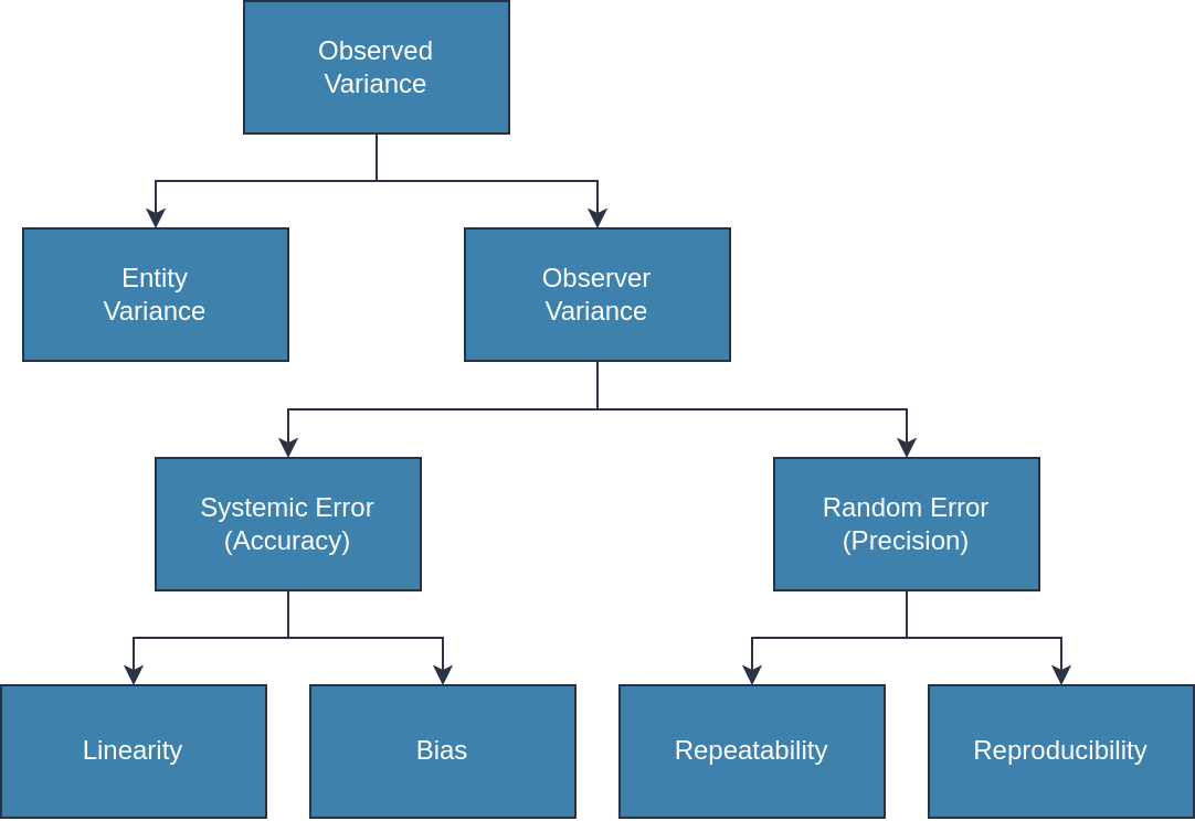
(Random) measurement error can be decomposed in to repeatability, and reproducibility.
We can use a gauge study to to separate out these effects and answer some important questions about:
- Repeatability: Does the measuring device give consistent measurements for the same part?
- Reproducibility: Do different observers give consistent measurements of the same part?
- Is the instrument precise enough to detect differences between parts?
Setting Up a Gauge Study
In a crossed gauge study we have:
- $n_o$ observers measure
- $n_p$ parts, with
- $n_r$ replicates or repeat measurements.
By having multiple observers measure the same parts we can filter out the bias that any individual may have, and account for interaction of operator and part.
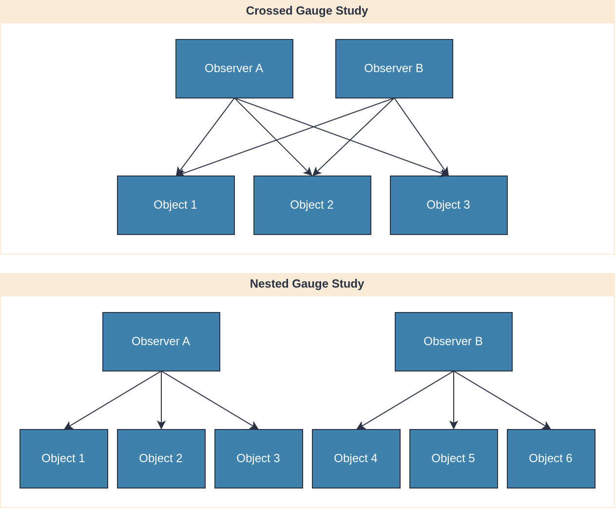
In a crossed gauge study, every observer measures every object or part.
Every observer measures every part multiple times. It is also important to randomise the order in which observations are taken to reduce any bias or systematic effects.
The table below shows how a data collection form for a gauge study should look. Programs like Minitab can generate these automatically for you, though it is simple enough to create one in a spreadsheet.
| Standard Order | Randomised Order | Part Number | Observer | Replicate | Measurement |
|---|---|---|---|---|---|
| 3 | 1 | 3 | A | 1 | 38 |
| 21 | 2 | 1 | B | 1 | 37 |
| 14 | 3 | 4 | A | 2 | 38 |
| 13 | 4 | 3 | A | 2 | 37 |
| 53 | 5 | 3 | C | 2 | 37 |
Calculations
1. Total Mean
We first begin by calculating the mean of all measurements:
\[\bar{y}_{\cdot\cdot\cdot} = \frac{1}{n_o n_p n_r}\sum_{i=1}^{n_o} \sum_{j=1}^{n_p}\sum_{k=1}^{n_r} y_{ijk} \tag{3}\]This becomes our reference or anchor point for separating out the reproducibility and reliability.
2. Operator
We then compute operator means:
\[\bar{y}_{\cdot i\cdot} = \frac{1}{n_p n_r}\sum_{j=1}^{n_p}\sum_{k=1}^{n_r} y_{ijk}. \tag{4}\]Then we compute the (sample) variance for all the operator measurements:
\[s_o^2 = \frac{1}{n_o - 1}\sum_{i=1}^{n_o}\big(\bar{y}_{i \cdot \cdot } - \bar{y}_{\cdot \cdot \cdot})^2. \tag{5}\]3. Part
Next we compute the mean for each part:
\[\bar{y}_{\cdot j\cdot} = \frac{1}{n_o n_r}\sum_{i=1}^{n_o} \sum_{k=1}^{n_r} y_{ijk} \tag{6}\]and its accompanying variance:
\[s_p^2 = \frac{1}{n_p - 1} \sum_{j=1}^{n_p} \left(\bar{y}_{\cdot j\cdot} - \bar{y}_{\cdot\cdot\cdot}\right)^2. \tag{7}\]4. Operator-by-Part
Next we compute the mean effect between operators and parts:
\[\bar{y}_{ij\cdot} = \frac{1}{n_r} \sum_{k=1}^{n_r} y_{ijk} \tag{8}\]Now, computing the variance for the operator-by-part interaction is complicated. But consider that, when we take the average, we eliminate measurement error $e_{ijk}$ since its mean is zero:
\[\bar{y}_{ij\cdot} = \bar{y}_{\cdot\cdot\cdot} + o_i + p_j + (o\times p)_{ij}. \tag{9}\]We may then rearrange Eqn. (9) to obtain: \(\begin{align} (o\times p)_{ij} &\approx \bar{y}_{ij\cdot} - \overbrace{(\bar{y}_{i\cdot\cdot} - \bar{y}_{\cdot \cdot \cdot})}^{p_i} - \overbrace{(\bar{y}_{\cdot j\cdot} - \bar{y}_{\cdot \cdot \cdot})}^{o_j} - \bar{y}_{\cdot \cdot \cdot} \tag{10a}\\ &= \bar{y}_{ij\cdot} - \bar{x}_{i\cdot \cdot} - \bar{y}_{\cdot j \cdot} + \bar{y}_{\cdot \cdot \cdot} \tag{10b} \end{align}\)
Then the variance is computed as:
\[s_{op}^2 = \frac{1}{(n_o-1)(n_p -1)} \sum_{i=1}^{n_o}\sum_{j=1}^{n_p} \underbrace{(\bar{y}_{ij\cdot} - \bar{y}_{i\cdot\cdot} - \bar{y}_{\cdot j \cdot} + \bar{y}_{\cdot \cdot \cdot})}_{(o\times p)_{ij}} {}^2 . \tag{11}\]5. Instrument
Finally we can compute the instrument errors as the difference of any individual observation from the operator-by-part mean: \(e_{ijk} = y_{ijk} - \bar{y}_{ij\cdot}. \tag{12}\)
The interpretation here is that $\bar{y}_{ij\cdot}$ averages out any errors from individual operators or parts.
We compute the (sample) variance of the instrument error as:
\[s_e^2 = \frac{1}{n_o n_p (n_r - 1)} \sum_{i=1}^{n_o} \sum_{j=1}^{n_p} \sum_{k=1}^{n_r} \left(y_{ijk} - \bar{y}_{ij\cdot}\right)^2. \tag{13}\]6. Gauge R&R
Now having computed the variances for each source of error may determine the gauge repeatability and reliability.
The total variance of our gauge study $s^2$ is the sum of all the individual variances in which:
- $s_e^2$ is the repeatability of the instrument,
- $s_o^2 + s_{op}^2$ is the reproducibility, and
- $s_p^2$ is the process, or part-to-part variation.
The sum of the repeatability and reproducibility is, as you would have guessed, the Gauge R&R.
📝 NOTE: Programs like Minitab can perform this analysis for you. But, being a masochist, I learnt and programmed the math myself.
How Good is Your Gauge?
Number of Distinct Categories
Normally when you perform a gauge study with a program like Minitab it prints out statistical information, including something called “number of distinct categories”.
According to ChatGPT, and a few sources I read on the internet, this is computed as;
\[NDC = \frac{\sqrt{2} s_p}{s_{grr}}. \tag{15}\]A value of $NDC \ge 5$ is considered quite good.
Try as I might, I could not reverse engineer this equation, nor make any sense of the $\sqrt{2}$ on the numerator. From what I could determine, this is simply a heuristic.
In the proceeding section I will propose a more mathematically sound metric.
Better Metrics
Gauge Capability
For a process that produces goods or services, the capability is defined as the upper specification limit (USL) minus the lower specification limit (LSL), divided by 6 standard deviations of the process variation:
\[C_p = \frac{USL - LSL}{6\sigma} \tag{16}\]A good process has $C_p \approx 1$. As shown in the diagram below, the specification limits are thus $\pm 3\sigma$ either side of the mean, or 99.7% of the process variation is within the specification limits.
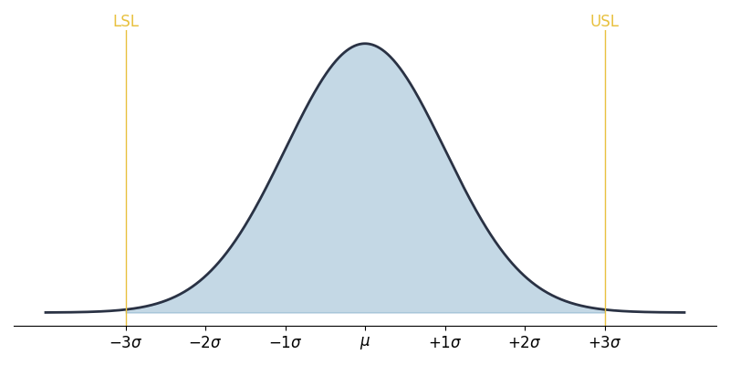
A $6\sigma$ process has upper and lower specification limits 3 standard deviations either side of the mean $\mu$.
We can extend this idea to our gauge. We can take the ratio of the process standard deviation over 6 times the gauge R&R:
\[C_{gauge} = \frac{s_p}{6\cdot s_{grr}} \tag{17}\]That is, our process variation is 6 times larger than Gauge R&R. An excellent gauge will have $C_{gauge} \approx 1$.
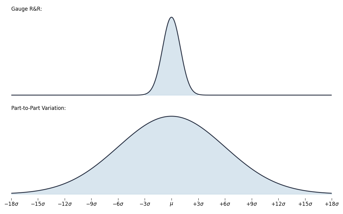
An excellent gauge will have 1/6 the of the process variation.
Gauge Resolution
Given the gauge variance, i.e. uncertainty in our measurement, what is the minimum value $\Delta p$ that it can detect? If we assume a Normal distribution, then we can use a z-score to determine to determine different confidence levels.
For example, a z-score of 1.96 equates to 95% probability, or confidence. We can solve the following equation to find the minimum detectable value with 95% confidence:
\[\begin{align} z = \frac{\Delta p}{s_{grr}} &= 1.96 \tag{18a}\\ \Delta p &= 1.96 \cdot s_{grr} \tag{18b} \end{align}\]We can do this for other values as well.
| Z-Score | Confidence Level |
|---|---|
| 1.645 | 90% |
| 1.96 | 95% |
| 2.576 | 99% |
Any value below the gauge resolution we cannot be certain is due to measurement error.
Case Studies
Below are gauge studies conducted on 2 different sets of scales:
- My kitchen scales, and
- Expensive scales in my laboratory at work.
The gauge study consisted of measuring:
- 10 bags of M&Ms ($n_p = 10$), between
- 3 people ($n_o = 3$), with
- 2 replicates ($n_r = 2)$
for a total of $10 \times 3 \times 2 = 60$ measurements. Measurement order was randomised for each study to reduce bias.
If you want to perform your own data analysis, you can find all the raw data in CSV format for:
Kitchen Scales
I bought my kitchen scales from Kasanova when I was living in Italy. The resolution on the digital display is a minimum of 1g.
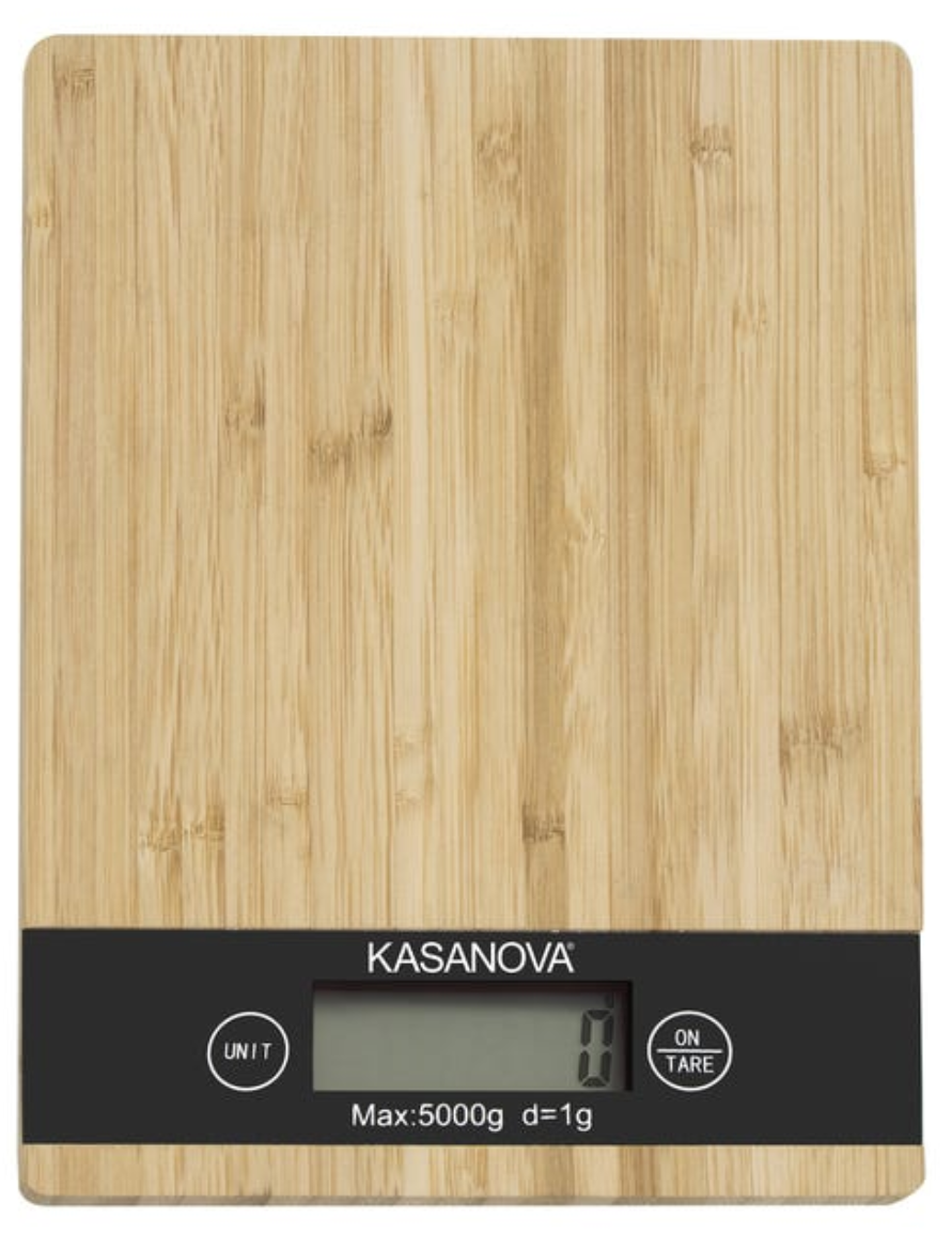
Bilancia elettronica Bambù da cucina, portata 5 kg
Below is a stem and leaf plot of the measurements taken during the gauge study:
| Stem | Leaves |
|---|---|
| 3 | 6 7 7 7 7 7 7 7 7 7 7 7 7 7 7 7 7 7 7 7 7 8 8 8 8 8 8 8 8 8 8 8 8 8 8 8 8 8 8 8 8 8 8 8 9 9 9 9 9 9 9 9 9 9 9 9 9 |
| 4 | 0 0 0 |
The median value is 37g; this is 1g higher than advertised. There is also an outlier of 40g.
The table below shows the results of the gauge study:
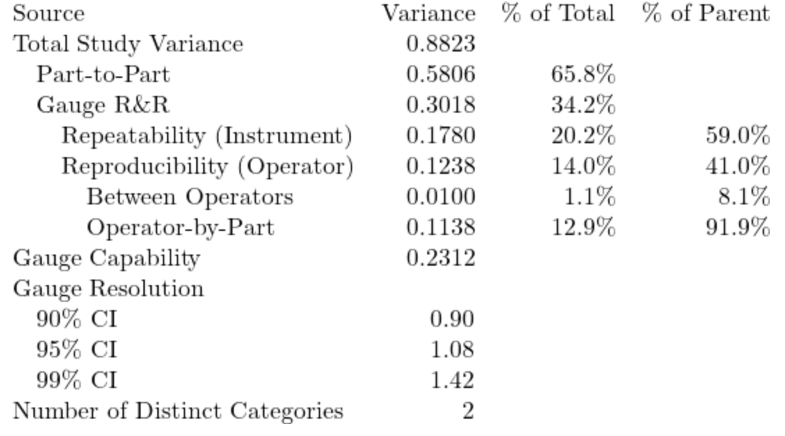
The estimated gauge capability $C_{gauge} \approx 0.2 < 1$ which is not good. Likewise, the number of distinct categories was estimated to be $2 < 5$ which again, is not good.
The estimated resolution is about 1.4 grams (99% confidence), so probably closer to 2g if we were to be conservative and round up.
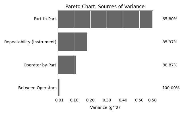
The pareto chart below show the cumlative contribution for the sources of measurement variance. There is significant variance coming from the scales themselves; the repeatability.
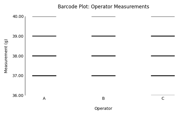
When we plot individual observations by operator we can see that they line up with the 1g resolution of the scales themselves. Not much insight here.
Plotting the observations by part reveals another story. Despite the low resolution of the scales, the part measurements are quite inconsistent across operators. Look at bag no. 7 for example. There was a 2g discrepency between Operator A and Operator C. Operators weren’t even able to measure the same part consistently.

Conclusion: These scales are not good if we want to control the weight of M&M bags in a production line!
Lab Scales
The lab scales are from Kern & Sohn, and are about 20 times more expensive (thankfully I didn’t have to pay for them!).
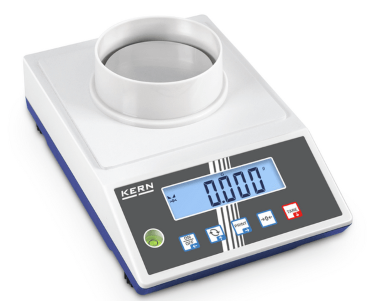
Kern PCB Economy Precision Balance
The digital display has a resolution of 0.001g (remember this for later).
The stem and leaf plot below shows the distribution of measurements obstained during the gauge study. Immediately we can see, due to the higher resolution, a wider distriubtion of values. But interestingly, the median lies in the 37g range:
| Stem | Leaves |
|---|---|
| 37 | .136 .138 .138 .139 .140 .142 .143 .146 .146 .146 .146 .148 .507 .511 .516 .521 .523 .523 .532 .533 .533 .537 .542 .572 .842 .849 .850 .853 .854 .855 .885 .885 .894 .894 .894 .898 .945 .956 .962 .962 .964 .974 |
| 38 | .117 .117 .118 .119 .121 .122 |
| 39 | .429 .429 .433 .436 .442 .444 .475 .476 .476 .485 .486 .489 |
The table below shows the results of the gauge study:
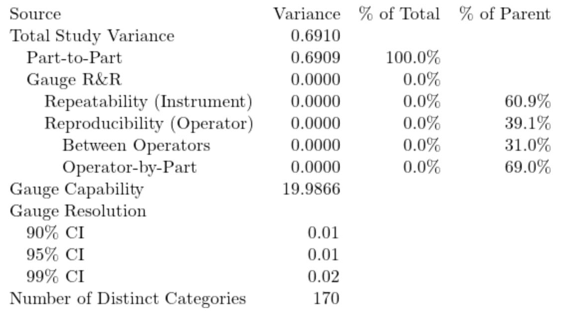
The estimated gauge capability is $C_{gauge} \approx 20 \gg 1$, so this is a very good gauge. The distinct number of categories is also 170 $\gg$ 5, which supports this.
My estimated resolution of the gauge is 0.02g (99% confidence), so it seems that the 3rd decimal place.
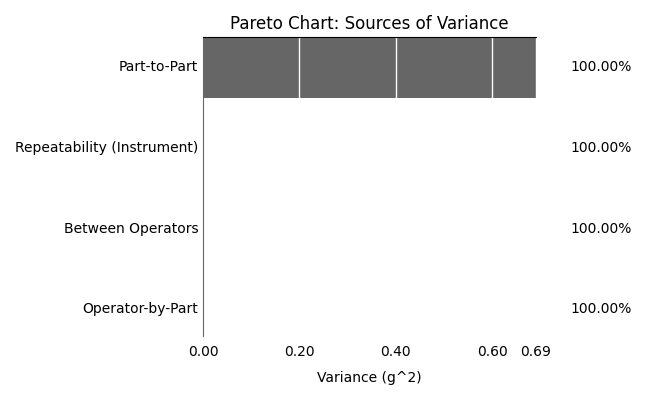
The pareto chart below shows that, within the study, all the variance in the measurements were due to the differences in bags themselves. This is in stark contrast to the kitchen scales is not useful.
When we look at observations by operator, we get consistent distributions:
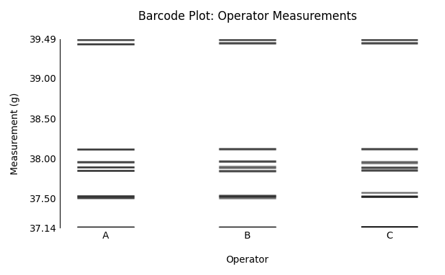
And when we examine operator-by-part, we can see that all operators are measuring each part consistently. So, unlike the kitchen scales, this measuring device does not appear to be susceptible to operator idiosynchrasies.

Conclusions: These scales are extremely precise. Probably too precise for weighing bags of M&Ms. It means we could use a potentially cheaper set of scales for controlling production.
Key Takeaways
A measurement or observation of a quantity can have multiple sources of variance:
- The thing itself being observed,
- The measuring device, or
- The thing doing the observing (the observer).
By performing a systematic gauge study we can isolate these sources of error.
We have also seen that the interaction between operator and the measuring device can have an effect on measurement variance, as evinced by the study of my kitchen scales.
Moreover, it is important to select a gauge that is appropriate to the measuring task. My kitchen scales are sufficient for cooking at home, but probably not for a production line. Conversely, the lab scale are probably too_ precise for such a task
It seems that Mars Inc. (who produce M&Ms) are over-filling their bags. Value for money!
I also now have a lot of chocolate to eat.
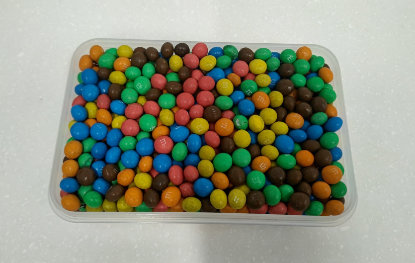
Statistics can be fun, and delicious.
I made the graphs for this post using my newly released tufteplotlib package for Python.